Deterministic setting

When dealing with large populations deterministic models are often used. In deterministic compartmental models, the transition rates from one compartment to another are mathematically expressed as derivatives. Hence the model is formulated using ordinary differential equations (ODE). A closed population is assumed at all times \(t\), then \(P(t)=S(t)+I(t)+R(t)\).

• \(\frac{dS(t)}{dt} = - \beta S(t)\frac{I(t)}{P(t)}\)
• \(\frac{dI(t)}{dt} = \beta S(t)\frac{I(t)}{P(t)} - \gamma I(t)\)
• \(\frac{dR(t)}{dt} = \gamma I(t)\)

Here are two example of deterministic modelling with and without birth and death process in the compartments.

##package
library(deSolve)

##################################################
### Basic model SIR simulations
###################################################

##function
sir <- function(time, state, parameters) {
  with(as.list(c(state, parameters)), {
    dS <- -beta * S * I
    dI <- beta * S * I - gamma * I
    dR <- gamma * I
    
    return(list(c(dS, dI, dR)))
  })
}

##############################################################################
init <- c(S = 1-1e-6, I = 1e-6, 0.0)
parameters <- c(beta = 0.15, gamma = 0.005)
times <- seq(0, 1000, by = 1)
out <- as.data.frame(ode(y = init, times = times, func = sir, parms = parameters))
out$time <- NULL

par(cex=1.5)

matplot(times, out, type = "l", xlab = "Time", ylab = "Population", main = "SIR Model", lwd = 1, lty = 1, bty = "l", col = 2:4)
legend(x = 500,y = 0.6,c("Susceptibles", "Infecteds", "Recovereds"), pch = 16, col = 2:4)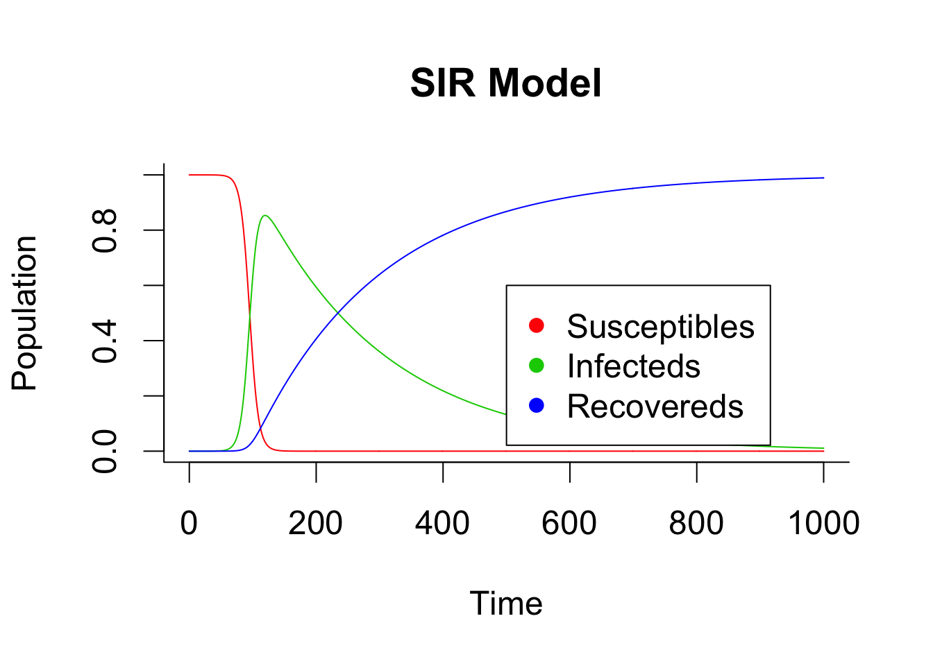

##################################################
### Model SIR with birth and dead rate 
###################################################


sir_bd <- function(time, state, parameters) {
  with(as.list(c(state, parameters)), {
    dS <- birth - beta*S*I - death*S
    dI <- beta*S*I - gamma*I - death*I
    dR <- gamma*I - death*R
    
    return(list(c(dS, dI, dR)))
  })
}


##############################################################################
init <- c(S = 1-1e-6, I = 1e-6, R = 0.0)
parameters <- c(beta = 0.15, gamma = 0.005, birth =0.001, death=0.001)
times <- seq(0, 1000, by = 1)
out <- as.data.frame(ode(y = init, times = times, func = sir_bd, parms = parameters))
out$time <- NULL

matplot(times, out, type = "l", xlab = "Time", ylab = "Population", main = "SIR Model including birth and death rates", lwd = 1, lty = 1, bty = "l", col = 2:4)
legend(x = 500,y = 0.6,c("Susceptibles", "Infecteds", "Recovereds"), pch = 16, col = 2:4)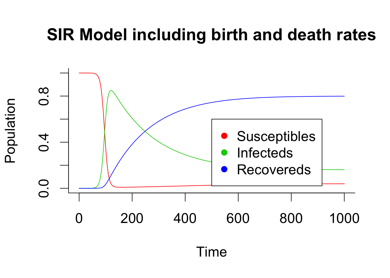

Stochastic modelling

A stochastic SIR model is defined analogously as the deterministic model. A closed homogeneous population is assumed, and \(S(t)\), \(I(t)\) and \(R(t)\) have the same definition as in the deterministic setting. As done previously, birth and death are ignored in this simple setting. The dynamic of the model is defined as follows. Infectives have contact with susceptibles at a constant rate \(\beta\). Contacts are mutually independent. Any susceptible which is in contact with an infected individual immediately becomes infective and starts spreading the disease following the same rules. Infected individuals remain infectious for a random amount of time governed by an infections period distribution after which they stop being infectious and recover. The infectious periods are defined to be independent and identically distributed (also independent of the contact processes). The exponential distribution with intensity parameter \(\gamma\) has received special attention in the literature, because the resulting model is Markovian. A stochastic process is said to be a Markov process or have the markov property if the conditional probability of the future state conditional on both present and past states depends only on the present state of the process.

A simple and efficient algorithm to simulate a stochastic model is the Gillespie algorithm. This algorithm assumes that all possible transitions between compartments occur independently and are simulated at each time step with constant probability per unit time that depends on the current state of the system (i.e the number of individual in each compartment). The idea is to sample the next time event from an exponential distribution. Then, the event is randomly chosen amongst the possible transitions between compartments with probabilities proportional to their individual rates. The code below shows two realizations for a small and a large population of a stochastic SIR model simulated by a Gillespie algorithm.

parms=c(m=0,b=0.02,v=0.1,r=0.3)

# define how state variables S, I and R change for each process
processes <- matrix(c(1,1,1,
                      -1,0,0,
                      0,-1,0,
                      0,0,-1,
                      -1,1,0,
                      0,-1,0,
                      0,-1,1), nrow=7, ncol=3, byrow = TRUE,
                    dimnames=list(c("birth",
                                    "death.S",
                                    "death.I",
                                    "death.R",
                                    "infection",
                                    "death.infec",
                                    "recovery"),
                                  c("dS","dI","dR")))

##import necessary files/fct
source(file="RFun/gillespie_fct_R.R")

##small population
initial.state=c(S=97, I=3, R=0)

res<-gillespie(parms=parms, X0=initial.state, time.window=c(0,1000), processes=processes,pb = FALSE)
par(cex=1.5)
matplot(x = res[,1], y = res[,-1], type = "l", lty = 1, xlab = "Time", ylab = "Population",col = 2:4, ylim=c(0,100), xlim=c(0,10), main="One realization of a stochastic model \n for S(0)=97, I(0)=3, R(0)=0")
legend(x=6,y=50,c("Susceptibles", "Infecteds", "Recovereds"), pch = 16, col = 2:4)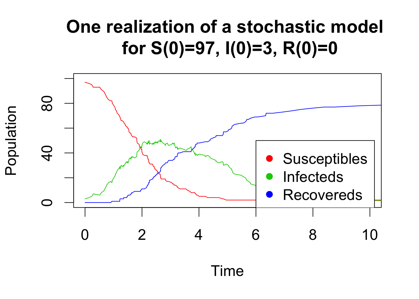

##huge population
initial.state=c(S=997, I=3, R=0)

res<-gillespie(parms=parms, X0=initial.state, time.window=c(0,10000), processes=processes,pb = FALSE)
matplot(x = res[,1], y = res[,-1], type = "l", lty = 1, xlab = "Time", ylab = "Population",col = 2:4, ylim=c(0,1000), xlim=c(0,10), main="One realization of a stochastic model \n for S(0)=997, I(0)=3, R(0)=0")
legend(x=6,y=500,c("Susceptibles", "Infecteds", "Recovereds"), pch = 16, col = 2:4)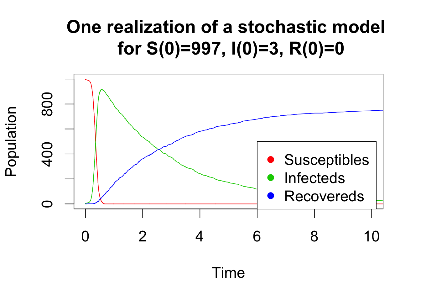

In a next post I will comment on the code of the parallel gillespie R function …