This post is highly inspired by this post and this post. Here is the necessary code to produce those graphs (be aware that it is time and memory consuming!).
On June 10 2013, RStudio provides CRAN mirror logs download from 2012-10-01. Then it is possible to analyze this rich and huge amount of data. On an individual level, one can track the popularity of their (preferred package). Here one can track the number of download of the three most downloaded R packages.
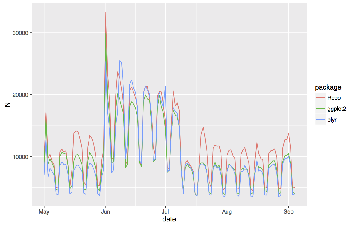
Here is the daily counts for the three most downloaded R packages, for May the 1 to September the 4th 2016. As one can see, there is an obvious weekly seasonality.

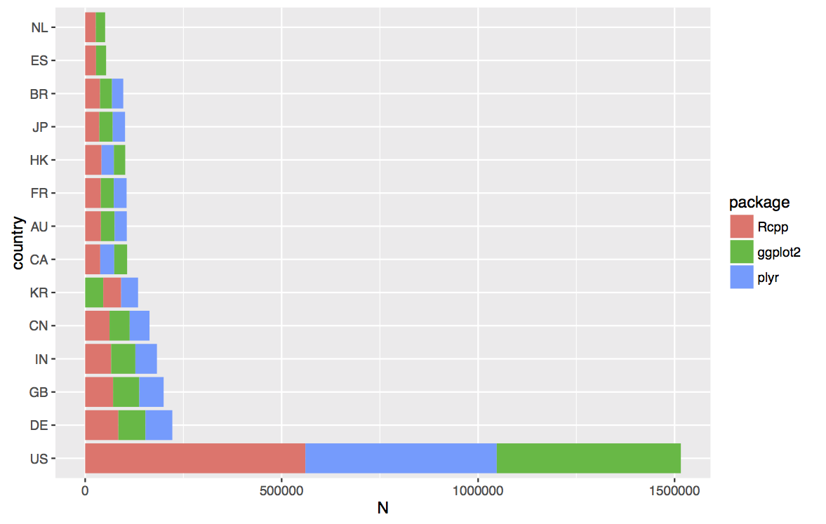
Here is the ordered total number of download per country for the same period. Rcpp seems to be the most used R package in all countries except Korea.

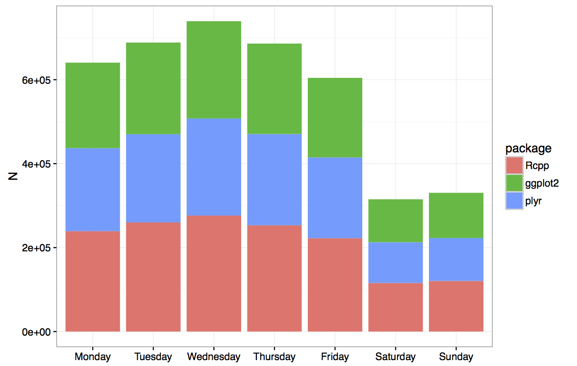
Here is the total count over the week days for this period. As one can see, number of downloads decreases of about a half during the weekend.

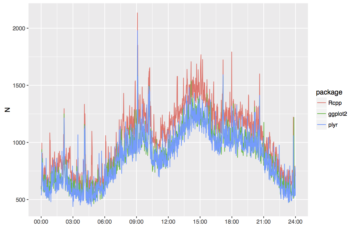
Finally, this graph represents the instantly (smoothed by minute) number of downloads in standardized UTC. As one can see, less downloads during night and lunch time.

Below is the necessary code to extract, manipulate and plot the data.
###########################################################################
##Gilles Kratzer
##Analysis on CRAN Rstudio log files in order to compute to the number of downloads
##History :
## --2016/09/06 document created
## --2016/09/09 adding material
## --2016/09/21 plotting data
###########################################################################

###########################################################################
##Purpose: Analysis of the downloads of R packages
##Highly inspired by https://www.r-bloggers.com/finally-tracking-cran-packages-downloads/
##Highly inspired by http://blog.kongscn.me/2015/05/15/r-packages-stats.html
###########################################################################

##cleaning
rm(list = ls())
graphics.off()

##packages
library(lubridate)
library(data.table)
library(dplyr)
library(tidyr)
library(dplyr)
library(ggplot2)


## ======================================================================
## Step 1: Download all log files
## ======================================================================


# Here's an easy way to get all the URLs in R
# It downloads only the missing files
# !!! very long !!!

start <- as.Date('2016-05-01')
today <- as.Date('2016-10-15')

all_days <- seq(start, today, by = 'day')

year <- as.POSIXlt(all_days)$year + 1900
urls <- paste0('http://cran-logs.rstudio.com/', year, '/', all_days, '.csv.gz')

# only download missing files
missing_days<-setdiff(as.character(all_days), tools::file_path_sans_ext(dir("../3m/"), TRUE))

dir.create("../3m/")
for (i in 1:length(missing_days)) {
  print(paste0(i, "/", length(missing_days)))
  download.file(urls[i], paste0('../3m/', missing_days[i], '.csv.gz'))
}


## ======================================================================
## Step 2: Make a data table
## ======================================================================

#!!! time and memory consuming

DT = data.table()
files = list.files("../3m", pattern='*.gz', full.names=TRUE)

for (file in files){
  print(paste("Reading", file, "..."))
  dt = tbl_dt(read.csv(file, as.is=TRUE))
  dt = dt[, `:=`(datetime=ymd_hms(paste(date, time)),
                 r_version=as.factor(r_version),
                 r_arch=as.factor(r_arch),
                 r_os=as.factor(r_os),
                 package=as.factor(package),
                 date=NULL, time=NULL, ip_id=NULL, version=NULL)]
  DT = rbind(DT, dt)
}
rm(dt)
DT = tbl_dt(DT)
setkey(DT, package, country)
save(DT, file="../3m/3m_final.RData")
gc() # !!!

## ======================================================================
## Step 3: Analysis
## ======================================================================

load(file = "../3m/3m_final.RData")

by_package = DT[, .N, keyby=package][order(-N)]

# Top downloads
by_package

top3 = DT[.(c("Rcpp","plyr", "ggplot2"))]
top3[, `:=`(date=as.Date(datetime))]

top3_stat = top3[, .N, by=.(package, date)]
qplot(x=date, y=N, data=top3_stat, geom='line', color=package)

ggsave(filename = "dowloads_top3.pdf")

by_package <- DT[, .N, keyby=package][order(-N)]

top3[, `:=`(date=as.Date(datetime))]
pack_stat<-top3[, .N, by=.(package, date)]
qplot(x=date, y=N, data=pack_stat, geom='line', color=package)

ggsave(filename = "dowloads.pdf")

##country
pack_stat<-top3[,.N,keyby=.(country, package)][order(-N)]
pack_stat_count_country<-top3[,.N,keyby=.(country)][order(-N)]

pack_stat$country<-factor(x = pack_stat$country,levels = pack_stat_count_country$country)
m = ggplot(pack_stat[1:40], aes(x=country, y=N, fill=package))
m + geom_bar(stat="identity") + coord_flip()
ggsave(filename = "country_dowloads_top3.pdf")

##Download per day
top3$Weekdays <- weekdays(top3$datetime)

pack_stat<-top3[, .N, by=.(package, Weekdays)]
pack_stat$Weekdays<-factor(pack_stat$Weekdays, levels = c("Monday", "Tuesday", "Wednesday", "Thursday",
                                                          "Friday", "Saturday","Sunday"))
ggplot(aes(x=Weekdays, y=N, fill=package), data=pack_stat)+
  geom_bar(stat="identity")+
  theme_bw()+
  xlab(NULL)

ggsave(filename = "downloads_weekdays_top3.pdf")

##downloads per minutes
top3$specific_time <- hour(top3$datetime)+ minute(top3$datetime)/60

pack_stat<-top3[, .N, by=.(package, specific_time)]
qplot(x=specific_time, y=N, data=pack_stat, geom='line',color=package)+
  scale_x_continuous(breaks = c(0,3,6, 9, 12, 15,18,21,24), labels=c(
                                          "00:00",
                                          "03:00",
                                          "06:00",
                                          "09:00",
                                          "12:00",
                                          "15:00",
                                          "18:00",
                                          "21:00",
                                          "24:00"))+
  xlab(NULL)

ggsave(filename = "downloads_hour_top3.pdf")